Auto-Correlation and Echo Cancellation Overview

In this experiment you use the correlation of two sequences to solve a simple echo cancellation problem. The correlation of sequences y(n) and z(n) is another sequence, say R_yz(n), that is defined by

R_yz(n) = y(n) * z(-n)

That is, it is computed by evaluating the convolution of y(n) with the time-reversed version of z(n). The correlation serves as a useful measure of similarity between two sequences (and is actually used in pattern recognition applications).

When both sequences y(n) and z(n) are identical, we refer to the resulting correlation sequence as the auto-correlation sequence. Therefore, the auto-correlation sequence of y(n) is simply the convolution of y(n) with y(-n), and is denoted by

R_y(n) = y(n) * y(-n)

Now consider a signal y(n) that is obtained as the sum of a sequence x(n) and its delayed and scaled version, ax(n-N),

y(n) = x(n) + a . x(n-N)

where a is the amplitude of an echo x(n-N) and N is the delay in samples. Given measurements of y(n), we are interested in estimating the delay N of the echo. In the sequel we assume that the original sequence x(n) starts at time n=0. That is, x(n) is zero for n<0.

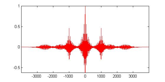
Due to the form of y(n), its autocorrelation function can be shown to have peak values at the time instants n=0, n=N, and n=-N. [You are asked to establish this fact in the exercises.] We show below a plot of the normalized auto-correlation function (or sequence) of a signal y(n) with an echo characterized by a =0 .8 and N=1000. [The function is normalized so that its peak value at n=0 is unity.] It is clear from the plot that there are peaks at the samples 0, 1000, and -1000.

Therefore, from a plot of the auto-correlation function we can determine the delay N. We assume a is known (methods for estimating a are beyond the scope of this exercise). Now given a and N, their values can be used to remove the echo and recover the original signal. This can be achieved in several ways. We explain two of them here. Depending on your background at this stage of the course, it might be easier for you to follow one method or another.

Time-Domain Method

First recall that we are assuming that the original sequence x(n) starts at time n=0. That is, x(n) is zero for n<0. This shows that the first N samples of x(n) and y(n) coincide,

x(n) = y(n) , for n<N.

We still need to recover the values of x(n) for time instants larger than or equal to N. For this purpose, we simply note that

y(N) = x(N) + a x(0) ,

so that x(N) can be recovered from

x(N) = y(N) - a x(0) .

Likewise, for values of n larger than N we employ successively the following relation,

x(n) = y(n) - a x(n-N),

Tranfer-Function Method

We can describe the recovery of x(n) in the transfer function domain as well. Indeed, note that the transfer function from x(n) to y(n) is FIR and given by

H(z) = 1 + az^{-N}

It follows that the transfer function from y(n) to x(n) is IIR and given by 1/H(z), namely

X(z)/Y(z) = 1/H(z)

That is,

X(z) = Y(z)/H(z) .

This means that we need to filter the observed signal y(n) through the filter 1/H(z) in order to recover x(n). This step can be achieved by using the 'filter' command of MATLAB.