A HMM consists of a number of states. Each state ![]() has an associated
observation probability distribution
has an associated
observation probability distribution
![]() which
determines the probability of generating observation
which
determines the probability of generating observation
![]() at
time
at
time ![]() and each pair of states
and each pair of states ![]() and
and ![]() has an associated
transition probability
has an associated
transition probability ![]() . In HTK the entry state
. In HTK the entry state ![]() and
the exit state
and
the exit state ![]() of an
of an ![]() state HMM are non-emitting.
state HMM are non-emitting.
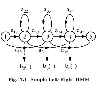
Fig. ![]() shows a simple left-right HMM with five states in
total. Three of these are emitting states and have output probability
distributions associated with them. The transition matrix for
this model will have 5 rows and 5 columns. Each row will sum to one
except for the final row which is always all zero since no
transitions are allowed out of the final state.
shows a simple left-right HMM with five states in
total. Three of these are emitting states and have output probability
distributions associated with them. The transition matrix for
this model will have 5 rows and 5 columns. Each row will sum to one
except for the final row which is always all zero since no
transitions are allowed out of the final state.
HTK is principally concerned with continuous
density models in which each observation probability distribution
is represented by a mixture Gaussian density. In this case,
for state ![]() the probability
the probability
![]() of generating
observation
of generating
observation
![]() is given by
is given by
HTK also supports discrete probability distributions in which case
In addition to the above, any model or state can have an
associated vector of duration parameters
![]() 7.1.
Also,
it is necessary to specify the kind of the observation
vectors, and the width of the observation vector in each stream.
Thus, the total information needed to define a single HMM is
as follows
7.1.
Also,
it is necessary to specify the kind of the observation
vectors, and the width of the observation vector in each stream.
Thus, the total information needed to define a single HMM is
as follows
![$\displaystyle b_{j}({\mbox{\boldmath$o$}}_t) = \prod_{s=1}^S \left[ \sum_{m=1}^...
...ox{\boldmath$\mu$}}_{jsm}, {\mbox{\boldmath$\Sigma$}}_{jsm}) \right]^{\gamma_s}$](img216.png)
![$\displaystyle b_{j}({\mbox{\boldmath$o$}}_t) = \prod_{s=1}^S \left\{ P_{js}[v_s({\mbox{\boldmath$o$}}_{st})] \right\}^{\gamma_s}$](img218.png)