Discriminative Parameter Re-Estimation Formulae

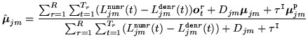
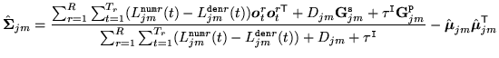
For both MMI and MPE training the estimation of the model parameters are based on variants of the Extended Baum-Welch (EBW) algorithm. In HTK the following form is used to estimate the means and covariance matrices^8.3

$$\hat{{\mbox{\boldmath$\mu$}}}_{jm} = \frac{ \sum_{r=1}^R \sum_{t=... ...T_r} (L^{{\tt num}r}_{jm}(t) - L^{{\tt den}r}_{jm}(t)) + D_{jm} + \tau^{\tt I}}$$ (8.13)

and

$$\hat{{\mbox{\boldmath$\Sigma$}}}_{jm} = \frac{ \sum_{r=1}^R \sum_... ...ox{\boldmath$\mu$}}}_{jm}\hat{{\mbox{\boldmath$\mu$}}}^{\scriptstyle\sf T}_{jm}$$ (8.14)

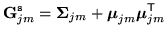
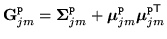
where

$${\bf G}_{jm}^{\tt s} = {{\mbox{\boldmath$\Sigma$}}}_{jm} + {{\mbox{\boldmath$\mu$}}}_{jm}{{\mbox{\boldmath$\mu$}}}_{jm}^{\scriptstyle\sf T}$$ (8.15)

$${\bf G}_{jm}^{\tt p} = {{\mbox{\boldmath$\Sigma$}}}^{\tt p}_{jm} ... ...\mu$}}}^{\tt p}_{jm}{{\mbox{\boldmath$\mu$}}}^{{\tt p}{\scriptstyle\sf T}}_{jm}$$ (8.16)

The difference between the MMI and MPE criteria lie in how the numerator, $L^{{\tt num}r}_{jm}(t)$, and denominator, $L^{{\tt den}r}_{jm}(t)$, ``occupancy probabilities'' are computed. For MMI, these are the posterior probabilities of Gaussian component occupation for either the numerator or denominator lattice. However for MPE, in order to keep the same form of re-estimation formulae as MMI, an MPE-based analogue of the ``occupation probability'' is computed which is related to an approximate error measure for each phone marked for the denominator: the positive values are treated as numerator statistics and negative values as denominator statistics.

In these update formulae there are a number of parameters to be set.

• Smoothing constant, $D_{jm}$: this is a state-component specific parameter that determines the contribution of the counts from the current model parameter estimates. In HMMIREST this is set at
  

  $$D_{jm} = \max\left\{ E\sum_{r=1}^R\sum_{t=1}^{T_r} L^{{\tt den}r}_{jm}(t),2D_{jm}^{\tt min} \right\}$$ (8.17)

  
  
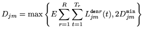
  where $D_{jm}^{\tt min}$ is the minimum value of $D_{jm}$ to ensure that ${\hat{{\mbox{\boldmath $\Sigma$}}}}_{jm}$ is positive semi-definite. $E$ is specified using the configuration variable E.

• I-smoothing constant, $\tau^{\tt I}$: global smoothing term to improve generalisation by using the state-component priors, ${{\mbox{\boldmath $\mu$}}}^{\tt p}_{jm}$ and ${{\mbox{\boldmath $\Sigma$}}}^{\tt p}_{jm}$. This is set using the configuration option ISMOOTHTAU.

• Prior parameters, ${{\mbox{\boldmath $\mu$}}}^{\tt p}_{jm}$ and ${{\mbox{\boldmath $\Sigma$}}}^{\tt p}_{jm}$: the prior parameters that the counts from the training data are smoothed with. These may be obtained from a number of sources. Supported options are;
  1. dynamic ML-estimates (default): the ML estimates of the mean and covariance matrices, given the current model parameters, are used.

  2. dynamic MMI-estimates: for MPE training the MMI estimates of the mean and covariance matrices, given the current model parameters, can be used. To set this option the following configuration entries must be added:

        MMIPRIOR = TRUE
        MMITAUI  = 50
     

     The MMI estimates for the prior can themselves make use of I-smoothing onto a dynamic ML prior. The smoothing constant for this is specified using MMITAUI.

  3. static estimates: fixed prior parameters can be specified and used for all iterations. A single MMF file can be specified on the command line using the -Hprior option and the following configuration file entries added

        PRIORTAU = 25
        STATICPRIOR = TRUE
     

     where PRIORTAU specifies the prior constant, $\tau^{\tt I}$, to be used, rather than the standard I-smoothing value.

The best configuration option and parameter settings will be task and criterion specific and so will need to be determined empirically. The values shown in the tutorial section of this book can be treated as a reasonable starting point. Note the grammar scale factors used in the tutorial are low compared to those often used in a typical large vocabulary speech recognition systems where values in the range 12-15 are used.

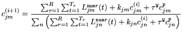
The estimation of the weights and the transition matrices have a similar form. Only the component prior updates will be described here. $c^{(0)}_{jm}$ is initialised to the current model parameter $c_{jm}$. The values are then updated 100 times using the following iterative update rule:

$${c}^{(i+1)}_{jm} = \frac{\sum_{r=1}^R \sum_{t=1}^{T_r}L_{jm}^{{\t... ..._{jn}^{{\tt num}r}(t) + k_{jn}c^{(i)}_{jn} + \tau^{\tt W}c^{\tt p}_{jn}\right)}$$ (8.18)

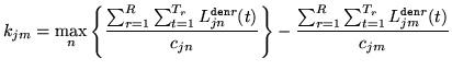
where

$$k_{jm} = \max_n\left\{\frac{\sum_{r=1}^R\sum_{t=1}^{T_r}L_{jn}^{{... ...} \right\} - \frac{\sum_{r=1}^R\sum_{t=1}^{T_r}L_{jm}^{{\tt den}r}(t)} {c_{jm}}$$ (8.19)

In a similar fashion to the estimation of the means and covariance matrices there are a range of forms that can be used to specify the prior for the component or the transition matrix entry. The same configuration options used for the mean and covariance matrix will determine the exact form of the prior.

For the component prior the I-smoothing weight, $\tau^{\tt W}$, is specified using the configuration variable ISMOOTHTAUW. This is normally set to 1. The equivalent smoothing term for the transition matrices is set using ISMOOTHTAUT and again a value of 1 is often used.