Let each spoken word be represented by a sequence of speech vectors or observations
![]() , defined as
, defined as
| (1.1) |
I
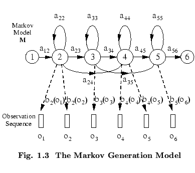
n HMM based speech recognition, it is assumed that the sequence of
observed speech vectors corresponding to each word is generated
by a Markov model as shown in Fig. ![]() .
A Markov model is a finite state machine which changes state
once every time unit and each time
.
A Markov model is a finite state machine which changes state
once every time unit and each time ![]() that a state
that a state ![]() is entered, a
speech vector
is entered, a
speech vector
![]() is generated from the probability density
is generated from the probability density
![]() . Furthermore, the transition from state
. Furthermore, the transition from state ![]() to state
to state ![]() is also probabilistic and is governed by the discrete probability
is also probabilistic and is governed by the discrete probability ![]() .
Fig.
.
Fig. ![]() shows an example of this process where the six state
model moves through the state sequence
shows an example of this process where the six state
model moves through the state sequence
![]() in
order to generate the sequence
in
order to generate the sequence
![]() to
to
![]() . Notice that
in HTK, the entry and exit states of a HMM are non-emitting. This
is to facilitate the construction of composite models as explained in
more detail later.
. Notice that
in HTK, the entry and exit states of a HMM are non-emitting. This
is to facilitate the construction of composite models as explained in
more detail later.
The joint probability that
![]() is generated by the model
is generated by the model ![]() moving
through the state sequence
moving
through the state sequence
![]() is calculated simply as the product of the transition
probabilities and the output probabilities. So for the state sequence
is calculated simply as the product of the transition
probabilities and the output probabilities. So for the state sequence ![]() in
Fig.
in
Fig. ![]()
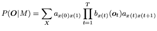
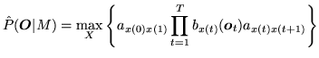
Given that ![]() is unknown, the
required likelihood is computed
by summing over all possible state
sequences
is unknown, the
required likelihood is computed
by summing over all possible state
sequences
![]() , that is
, that is
As an alternative to equation 1.5, the likelihood can be approximated by only considering the most likely state sequence, that is
Although the direct computation of equations 1.5 and 1.6
is not tractable, simple recursive procedures exist which allow
both quantities to be calculated very efficiently.
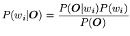
Before going any further, however, notice that if equation 1.2 is
computable then the recognition problem is solved. Given a set of models
![]() corresponding to words
corresponding to words ![]() , equation 1.2 is
solved by using 1.3 and assuming that
, equation 1.2 is
solved by using 1.3 and assuming that
All this, of course, assumes that the parameters
![]() and
and
![]() are known for each model
are known for each model ![]() . Herein lies the
elegance and power of the HMM framework. Given a set of training examples
corresponding to a particular model, the parameters of that model can be
determined automatically by a robust and efficient re-estimation
procedure. Thus, provided that a sufficient number of representative
examples of each word can be collected then a HMM can be constructed
which implicitly models all of the many sources of variability inherent
in real speech. Fig.
. Herein lies the
elegance and power of the HMM framework. Given a set of training examples
corresponding to a particular model, the parameters of that model can be
determined automatically by a robust and efficient re-estimation
procedure. Thus, provided that a sufficient number of representative
examples of each word can be collected then a HMM can be constructed
which implicitly models all of the many sources of variability inherent
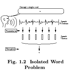
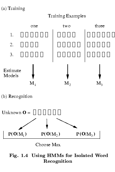
in real speech. Fig. ![]() summarises the use of HMMs
for isolated word recognition. Firstly, a
HMM is trained for each vocabulary word using a number of examples
of that word. In this case, the vocabulary consists of
just three words: ``one'', ``two'' and ``three''.
Secondly, to recognise some unknown word, the likelihood of
each model generating that word is calculated and the most likely
model identifies the word.
summarises the use of HMMs
for isolated word recognition. Firstly, a
HMM is trained for each vocabulary word using a number of examples
of that word. In this case, the vocabulary consists of
just three words: ``one'', ``two'' and ``three''.
Secondly, to recognise some unknown word, the likelihood of
each model generating that word is calculated and the most likely
model identifies the word.