Recognition and Viterbi Decoding

The previous section has described the basic ideas underlying HMM parameter re-estimation using the Baum-Welch algorithm. In passing, it was noted that the efficient recursive algorithm for computing the forward probability also yielded as a by-product the total likelihood $P({\mbox{\boldmath $O$}}\vert M)$. Thus, this algorithm could also be used to find the model which yields the maximum value of $P({\mbox{\boldmath $O$}}\vert M_i)$, and hence, it could be used for recognition.

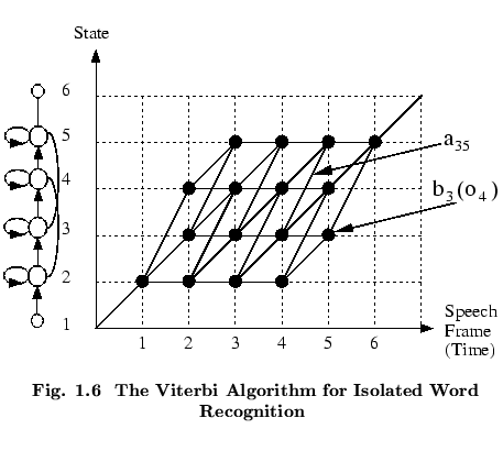
In practice, however, it is preferable to base recognition on the maximum likelihood state sequence since this generalises easily to the continuous speech case whereas the use of the total probability does not. This likelihood is computed using essentially the same algorithm as the forward probability calculation except that the summation is replaced by a maximum operation. For a given model $M$, let $\phi_j(t)$ represent the maximum likelihood of observing speech vectors ${\mbox{\boldmath $o$}}_1$ to ${\mbox{\boldmath $o$}}_t$ and being in state $j$ at time $t$. This partial likelihood can be computed efficiently using the following recursion (cf. equation 1.16)

$$\phi_j(t) = \max_i \left\{ \phi_i(t-1) a_{ij} \right\} b_j({\mbox{\boldmath$o$}}_t).$$ (1.27)

where

$$\phi_1(1) = 1$$ (1.28)

$$\phi_j(1) = a_{1j} b_j({\mbox{\boldmath$o$}}_1)$$ (1.29)

for $1<j<N$. The maximum likelihood $\hat{P}(O\vert M)$ is then given by

$$\phi_N(T) = \max_i \left\{ \phi_i(T) a_{iN} \right\}$$ (1.30)

As for the re-estimation case, the direct computation of likelihoods leads to underflow, hence, log likelihoods are used instead. The recursion of equation 1.27 then becomes

$$\psi_j(t) = \max_i \left\{ \psi_i(t-1) + log(a_{ij}) \right\} + log(b_j({\mbox{\boldmath$o$}}_t)).$$ (1.31)

This recursion forms the basis of the so-called Viterbi algorithm. As shown in Fig. , this algorithm can be visualised as finding the best path through a matrix where the vertical dimension represents the states of the HMM and the horizontal dimension represents the frames of speech (i.e. time). Each large dot in the picture represents the log probability of observing that frame at that time and each arc between dots corresponds to a log transition probability. The log probability of any path is computed simply by summing the log transition probabilities and the log output probabilities along that path. The paths are grown from left-to-right column-by-column. At time $t$, each partial path $\psi_i(t-1)$ is known for all states $i$, hence equation 1.31 can be used to compute $\psi_j(t)$ thereby extending the partial paths by one time frame.

$\parbox{100mm}{ \begin{center}\setlengt... ...e Viterbi Algorithm for Isolated Word Recognition} \end{center}\end{center} }$

This concept of a path is extremely important and it is generalised below to deal with the continuous speech case.

This completes the discussion of isolated word recognition using HMMs. There is no HTK tool which implements the above Viterbi algorithm directly. Instead, a tool called HVITE is provided which along with its supporting libraries, HNET and HREC, is designed to handle continuous speech. Since this recogniser is syntax directed, it can also perform isolated word recognition as a special case. This is discussed in more detail below.